A Biological Example
Suppose we are observing exponential growth $\dot{y} = \theta y$ but we don't know $\theta$ and wish to estimate it. We could assume $\theta \sim {\cal{N}}(\mu, \sigma^2)$ and use least squares or better something like Markov Chain Monte Carlo or Hamiltonian Monte Carlo and any observations to infer $\mu$ and $\sigma$. However, we might want to model that the further we go into the future, the less we know about $\theta$. We can write our system as as
$$ \begin{aligned} \mathrm{d}y & = \theta y\mathrm{d}t \\ \mathrm{d}\theta & = \sigma\mathrm{d}W_t \end{aligned} $$where $W_t$ is Brownian Motion.
Fokker-Planck
We can use the Fokker-Planck equation to convert a stochastic differential equation into a partial differential equation.
For our particular system we have
And since $\mu_1 = \theta y$, $\mu_2 = 0$ and $\sigma_y = 0$ this further simplifies to
We can note two things:
- This is an advection / diffusion equation with two spatial variables ($y$ and $\theta$).
- If $\sigma_\theta = 0$ then this is a transport (advection?) equation.
Notice that there is nothing stochastic about the biology but we express our uncertainty about the parameter by making it a time-varying stochastic variable which says the further we go into the future the less certain we are about it.
We are going to turn this into a Fokker-Planck equation which we can then solve using e.g. the method of lines. But before turning to Fokker-Planck, let's show that we can indeed solve a diffusion equation using the method of lines.
Warming Up
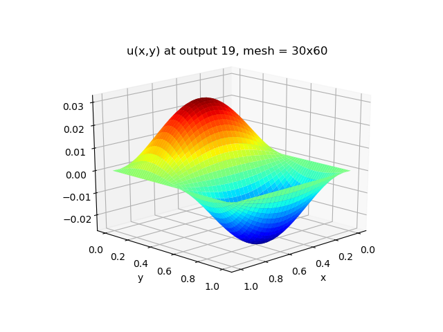
Let us solve the heat equation
with initial condition $u(0, x, y) = 0$ and stationary boundary conditions
$$ \frac{\partial u}{\partial t}(t, 0, y)=\frac{\partial u}{\partial t}(t, 1, y)=\frac{\partial u}{\partial t}(t, x, 0)=\frac{\partial u}{\partial t}(t, x, 1)=0 $$and a periodic heat source
$$ h(x, y)=\sin (\pi x) \sin (2 \pi y) $$This has analytic solution
$$ u(t, x, y)=\frac{1-e^{-\left(k_{x}+4 k_{y}\right) \pi^{2} t}}{\left(k_{x}+4 k_{y}\right) \pi^{2}} \sin (\pi x) \sin (2 \pi y) $$The spatial derivatives are computed using second-order centered differences, with the data distributed over $n_x \times n_y$ points on a uniform spatial grid.
We could try using Naperian functors and APL-like programming in Haskell via this library. But the performance is terrible (or it could be that the author's implementation was terrible). Moreover, applied mathematicans tend to think of everything as matrices and vectors. But flattening the above tensor operation into a matrix operation is not entirely trivial. Although the Haskell Ecosystem's support for symbolic mathematics is very rudimentary, we can use what there is to convince ourselves that we haven't made too many errors in the transcription.
{-# LANGUAGE DataKinds           #-}
{-# LANGUAGE OverloadedLists     #-}
{-# LANGUAGE ScopedTypeVariables #-}
{-# LANGUAGE FlexibleContexts    #-}
{-# LANGUAGE FlexibleInstances   #-}
{-# LANGUAGE MultiParamTypeClasses #-}
{-# LANGUAGE GADTs               #-}
{-# LANGUAGE TypeApplications    #-}
{-# LANGUAGE TypeOperators       #-}

import Data.Number.Symbolic
import qualified Data.Number.Symbolic as Sym
import Data.Proxy

import qualified Naperian as N
import qualified GHC.TypeLits as M
import           Data.Functor

import           Numeric.Sundials.ARKode.ODE
import           Numeric.LinearAlgebra

import           System.IO
We can re-write the semi-discretized equations in a tensor form from which we can derive an implementation.
Let's write down the tensor $A$ in Haskell
preA :: forall b m n . (M.KnownNat m, M.KnownNat n, Num b) =>
        N.Hyper '[N.Vector n, N.Vector m, N.Vector n, N.Vector m] b
preA = N.Prism $ N.Prism $ N.Prism $ N.Prism $ N.Scalar $
      N.viota @m <&> (\(N.Fin x) ->
      N.viota @n <&> (\(N.Fin w) ->
      N.viota @m <&> (\(N.Fin v) ->
      N.viota @n <&> (\(N.Fin u) ->
      (f m n x w v u)))))
        where
          m = fromIntegral $ M.natVal (undefined :: Proxy m)
          n = fromIntegral $ M.natVal (undefined :: Proxy n)
          f p q i j k l | i == 0               = 0
                        | j == 0               = 0
                        | i == p - 1           = 0
                        | j == q - 1           = 0
                        | k == i - 1 && l == j = 1
                        | k == i     && l == j = -2
                        | k == i + 1 && l == j = 1
                        | otherwise            = 0
We can concretize this to symbolic numbers
a :: forall a m n . (M.KnownNat m, M.KnownNat n, Floating a, Eq a) =>
      N.Hyper '[N.Vector n, N.Vector m, N.Vector n, N.Vector m] (Sym a)
a = N.binary (*) (N.Scalar $ var "a") preA
And do the same for the tensor $B$
preB :: forall b m n . (M.KnownNat m, M.KnownNat n, Num b) =>
        N.Hyper '[N.Vector n, N.Vector m, N.Vector n, N.Vector m] b
preB = N.Prism $ N.Prism $ N.Prism $ N.Prism $ N.Scalar $
      N.viota @m <&> (\(N.Fin x) ->
      N.viota @n <&> (\(N.Fin w) ->
      N.viota @m <&> (\(N.Fin v) ->
      N.viota @n <&> (\(N.Fin u) ->
      (f m n x w v u)))))
        where
          m = fromIntegral $ M.natVal (undefined :: Proxy m)
          n = fromIntegral $ M.natVal (undefined :: Proxy n)
          f :: Int -> Int -> Int -> Int -> Int -> Int -> b
          f p q i j k l | i == 0                   = 0
                        | j == 0                   = 0
                        | i == p - 1               = 0
                        | j == q - 1               = 0
                        | k == i     && l == j - 1 = 1
                        | k == i     && l == j     = -2
                        | k == i     && l == j + 1 = 1
                        | otherwise                = 0
b :: forall a m n . (M.KnownNat m, M.KnownNat n, Floating a, Eq a) =>
           N.Hyper '[N.Vector n, N.Vector m, N.Vector n, N.Vector m] (Sym a)
b = N.binary (*) (N.Scalar $ var "b") preB
We can check that our implementation matches the mathematical formula by rendering it as a $\LaTeX$.
ps :: forall m n . (M.KnownNat m, M.KnownNat n) =>
       [N.Vector n (N.Vector m ((Int, Int), Sym Double))]
ps = N.elements $ N.crystal $ N.crystal $ N.hzipWith (,) ss rhs
  where
    h = N.Prism $ N.Prism $ N.Scalar $
      N.viota @n <&> (\(N.Fin x) ->
      N.viota @m <&> (\(N.Fin w) ->
      var ("u_{" ++ show x ++ "," ++ show w ++ "}")))
    rhs = N.foldrH (+) 0 $ N.foldrH (+) 0 $ N.binary (*) preFoo h
    preFoo = N.binary (+) (a @Double @n @m) (b @Double @n @m)
    ss = N.Prism $ N.Prism $ N.Scalar $
         N.viota @n <&> (\(N.Fin x) ->
         N.viota @m <&> (\(N.Fin w) -> (x,w)))
eqns = mapM_ putStrLn $ zipWith (++) aaa bbb
  where
    aaa = concatMap (N.elements . N.Prism . N.Prism . N.Scalar) $
          fmap (fmap (fmap ((\(i, j)-> "u_{" ++ show i ++ show j ++ "} &= ") . fst))) x
    bbb = concatMap (N.elements . N.Prism . N.Prism . N.Scalar) $
          fmap (fmap (fmap ((++ " \\\\") . show . snd))) x
    x = ps @4 @3
eqns
And then getting our notebook to render the $\LaTeX$.
Now we have checked that our tensors look correct (at least for a particular and small tensor) we can try solving the system numerically
Spatial mesh size:
nx, ny :: Int
nx = 3
ny = 4
Heat conductivity coefficients:
kx, ky :: Floating a => a
kx = 0.5
ky = 0.75
x and y mesh spacing:
dx :: Floating a => a
dx = 1 / (fromIntegral nx - 1)
dy :: Floating a => a
dy = 1 / (fromIntegral ny - 1)
c1, c2 :: Floating a => a
c1 = kx/dx/dx
c2 = ky/dy/dy
Now we make the tensors more concrete by ensuring their elements come from Floating
bNum :: forall a m n . (M.KnownNat m, M.KnownNat n, Floating a) =>
        N.Hyper '[N.Vector n, N.Vector m, N.Vector n, N.Vector m] a
bNum = N.binary (*) (N.Scalar c1) preB
aNum :: forall a m n . (M.KnownNat m, M.KnownNat n, Floating a) =>
        N.Hyper '[N.Vector n, N.Vector m, N.Vector n, N.Vector m] a
aNum = N.binary (*) (N.Scalar c2) preA
Again we flatten the system into a matrix form so we can check everything looks as it should
bigA :: Matrix Double
bigA = fromLists $
       fmap (N.elements . N.Prism . N.Prism . N.Scalar) $
       N.elements $ N.crystal $ N.crystal $ N.binary (+)
       (aNum @Double @4 @3) (bNum @Double @4 @3)
bigA
h :: forall m n a . (M.KnownNat m, M.KnownNat n, Floating a) =>
                     N.Hyper '[N.Vector m, N.Vector n] a
h = N.Prism $ N.Prism $ N.Scalar $
     N.viota @n <&> (\(N.Fin x) ->
     N.viota @m <&> (\(N.Fin w) ->
     sin (pi * (fromIntegral w) * dx)
             * sin (2 * pi * (fromIntegral x) * dy)))
c :: Vector Double
c = fromList $ N.elements (h @3 @4 @Double)
t0, tf :: Double
t0 = 0.0
tf = 0.3

bigNt :: Int
bigNt = 20

dTout :: Double
dTout = (tf - t0) / (fromIntegral bigNt)

ts :: [Double]
ts = map (dTout *) $ map fromIntegral [1..bigNt]

sol :: Matrix Double
sol = odeSolveV SDIRK_5_3_4' Nothing 1.0e-5 1.0e-10 (const bigU') (assoc (nx * ny) 0.0 [] :: Vector Double) (fromList $ ts)
  where
    bigU' bigU = bigA #> bigU + c
main :: IO ()
main = do
  h1 <- openFile "Haskell.txt" WriteMode
  mapM_ (hPutStrLn h1) $ map (concatMap (' ':)) $ map (map show) $ toLists sol
  hClose h1
  mapM_ (\i -> putStrLn $ show $ sqrt $ (sol!i) <.> (sol!i) / (fromIntegral nx) / (fromIntegral ny)) ([0 .. length ts - 1] :: [Int])
main
The grid is unrealistically coarse. Let's check the Haskell implementation against a reference C implmentation with a better grid size.
nix-shell -I nixpkgs=https://github.com/NixOS/nixpkgs/archive/19.09.tar.gz
mpicxx ark_heat2D.cpp -lm -lsundials_arkode -lsundials_nvecparallel -o ark_heat2D
mpiexec -n 1 ./ark_heat2D
python plot_heat2D.py
We could run with more processors but it's easier to modify the python to work on the Haskell output if we don't.
nix-shell -I nixpkgs=https://github.com/NixOS/nixpkgs/archive/19.09.tar.gz
ghc -O2 -fforce-recomp Heat2D.hs -main-is Heat2D -o Heat2D
./Heat2D
python plot_heat2D.py